If you want to embed images in cells in Excel, you can do this in just a few steps. The feature is somewhat hidden and can be implemented in several ways.
Excel: Embedding images in cells – two approaches
If you want to embed an image in Excel, you have several options. You can also format both the image and the cell you want to use to fit your layout. If you can't access some features, you may need to remove Excel's read-only protection first.
- First, use Copy (shortcut: Ctrl+C) and Paste (shortcut: Ctrl+V) to copy the image you want from the clipboard into your Excel table. Alternatively, you can click on the image on the right and select the “Copy” option.
- Now reduce the size of the image so that it fits into the desired cell. To do this, simply drag the corners of the image to the correct size with the mouse. Alternatively, you can of course also adjust the column and row size.
- You can now use the Alt key to position the image in the correct cell.
- Then right-click on the image to open the context menu and select “Size and Properties”.
- Here, under “Properties”, you will find the option “depends on cell position and size”. This means that the image is adapted to the formatting and is taken into account when sorting the rows, for example.
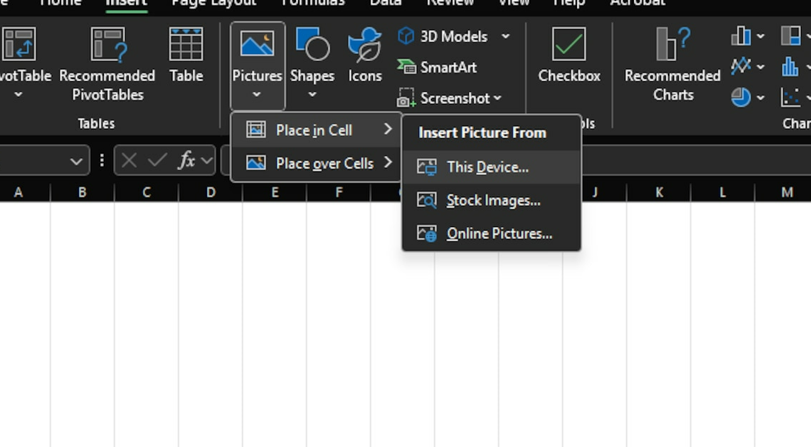
- Another option is the Insert function. First format a cell as you need it for the image and then click on it. Then click on “Insert”, then on Pictures in the menu bar and then select “Place in cell”. Now you have to select the source from which the image should be taken. Select your PC and then the image you want to place in Excel.