You can compare cells in Microsoft Excel using a simple formula. This will help you determine whether the data you have entered is true or false.
Comparing cells in Excel using the example of a player list
In our example, we want to determine which player found the correct solution. To do this, compare the solution you are looking for with the answers of the participants. The formula provided by Microsoft Excel for such calculations is called IDENTICAL. It allows you to find duplicate entries.
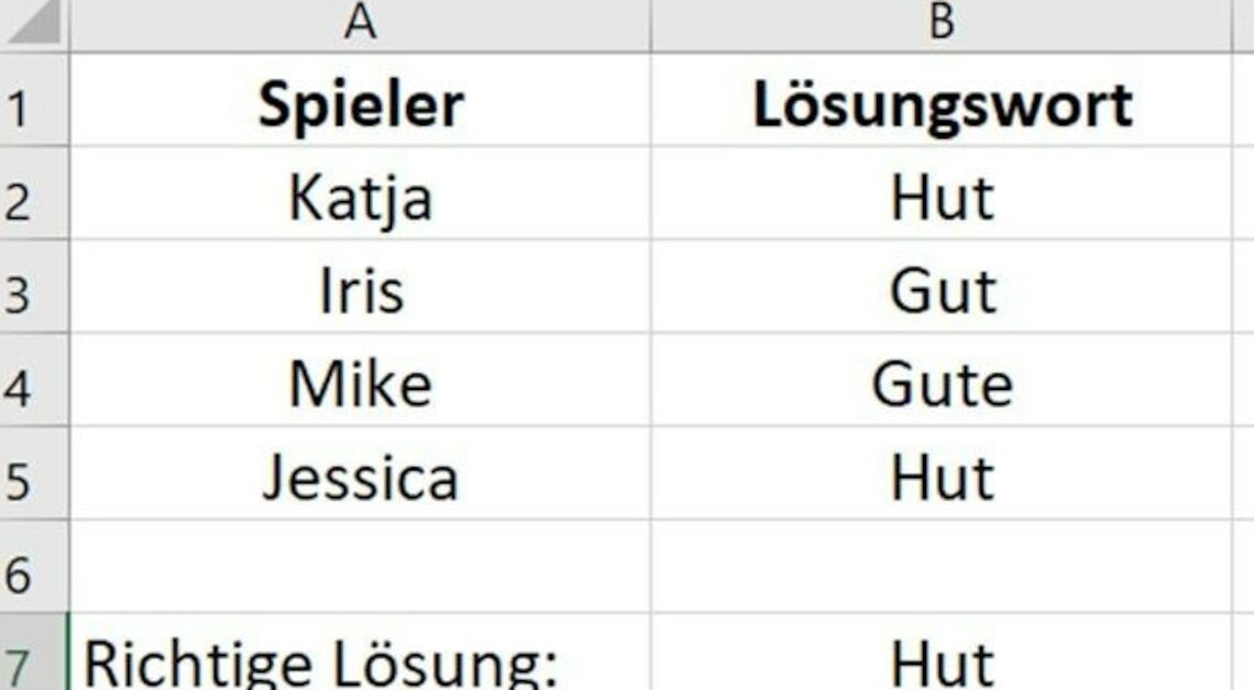
- In the example (see Figure 1 below), the names of the players were recorded in rows 2 to 5 in column A of an Excel spreadsheet. The players' solution words are listed in column B.
- Field B7 contains the correct solution. A formula must now be used to determine which player found the correct solution.
- To compare the player's answer with the correct answer, use the Excel function IDENTICAL. The syntax of the formula is: “IDENTICAL(Text1;Text2)”.
- This function compares the value of the cell specified as “Text1” with the value of the cell to be checked in “Text2”. Enter the formula in rows 2 to 5 of column C (see Figure 2).
- IDENTICAL is case sensitive. Normally Excel does not differentiate when checking cells. The following contents are the same for Excel: “Orange” and “orange”.
Comparing cells – step by step
To compare the player's answer with the result cell, let Microsoft Excel do the work. For large tables, the spreadsheet finds the right answers in no time.
- Click in cell C2. Now enter the IDENTICAL function as follows: =IDENTICAL(B2,B7).
- In the first argument of the formula (Text1) write down the first solution from cell B2. This is Katja's solution.
- As the second argument (Text2) you specify the cell with which you want to compare Katja's solution. In the example, this is cell B7.
- Confirm the formula with “Enter”. The result in cell C2 is “TRUE” because Katja's solution is correct.
- To check the results for all players, paste this formula into column C for the other players as well. Adjust the formulas to the appropriate cells. For Iris, Text1=B3, for Mike, B4, and for Jessica, B5.
- In column C you can see the solution. Both Katja and Jessica found the correct solution.
Compare the correct solution with a list
The IDENTICAL function also helps to perform comparisons from a long list of cells. This is useful, for example, for password comparisons or user names where differences between “user” and “user” are important. We'll stick with our example, but now use it as an array formula.
- In cell C7, enter the OR function: =OR(). It returns TRUE if the argument in parentheses is true, otherwise it returns FALSE.
- Click with the mouse in the editing line between the brackets of the function. This will display the required parameters. The formula requires at least one argument: “Boolean1”.
- Enter the function IDENTICAL as “Boolean1”: =OR(IDENTICAL()). Now click between the brackets of the IDENTICAL function to see the required parameters.
- In the first argument of the IDENTICAL function, enter the comparison value that contains the correct solution, here B7. End the input with a semicolon: =OR(IDENTICAL(B7;))
- As the second argument, select the cell range you want to compare with cell B7, here B2 to B5: =OR(IDENTICAL(B7;B2:B5)).
- Finish the formula as an array formula. To ensure that Excel recognizes the range, press the key combination: CTRL+SHIFT+ENTER. If you do not hold down the SHIFT key, Excel will give the answer “#VALUE!” instead of the result.
- Cell C7 now displays “TRUE” because there is at least one match to cell B7 in the cell range B2 to B5. In our example, at least one player found the correct solution using Microsoft Excel.