You can create a table of contents for worksheets in an Excel workbook either manually or using a macro. This way you can keep track of everything.
Create a table of contents for worksheets in an Excel workbook – manual method
Excel files with many worksheets can quickly become confusing. The solution is to set up a worksheet as a table of contents. You don't need to be able to program to do this.
- Open the document in Excel that you want to add a table of contents to. Point the mouse pointer at the first worksheet in the worksheet list. Then click the right mouse button once.
- Select “Insert” and click “Worksheet” in the “Insert” dialog box. It is located on the “General” tab. Confirm your selection with OK. Excel has now inserted a new, blank worksheet called “Sheet1” into the worksheet list for you.
- Right-click on the name of the new sheet and select “Rename”. You can now overwrite the existing name. Type “Table of Contents”.
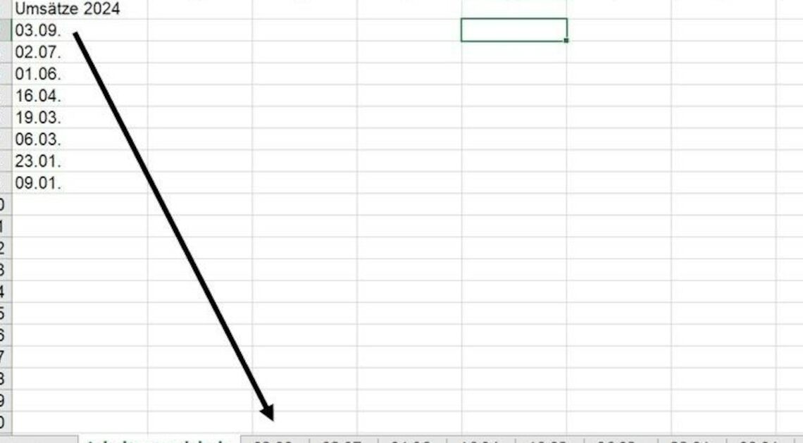
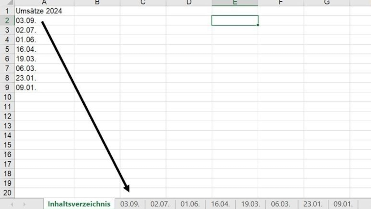
- Write a heading in cell A1, for example Sales 2024. From cell A2 onwards, enter the names of the individual worksheets one below the other (see Figure 1 below).
- Once you have entered all the names, click in cell A2 to insert the link to the worksheet. To do this, first click the “Insert” tab from the menu above.
- In the “Links” submenu (third from the right), left-click the link symbol once. This opens the “Insert Link” dialog.
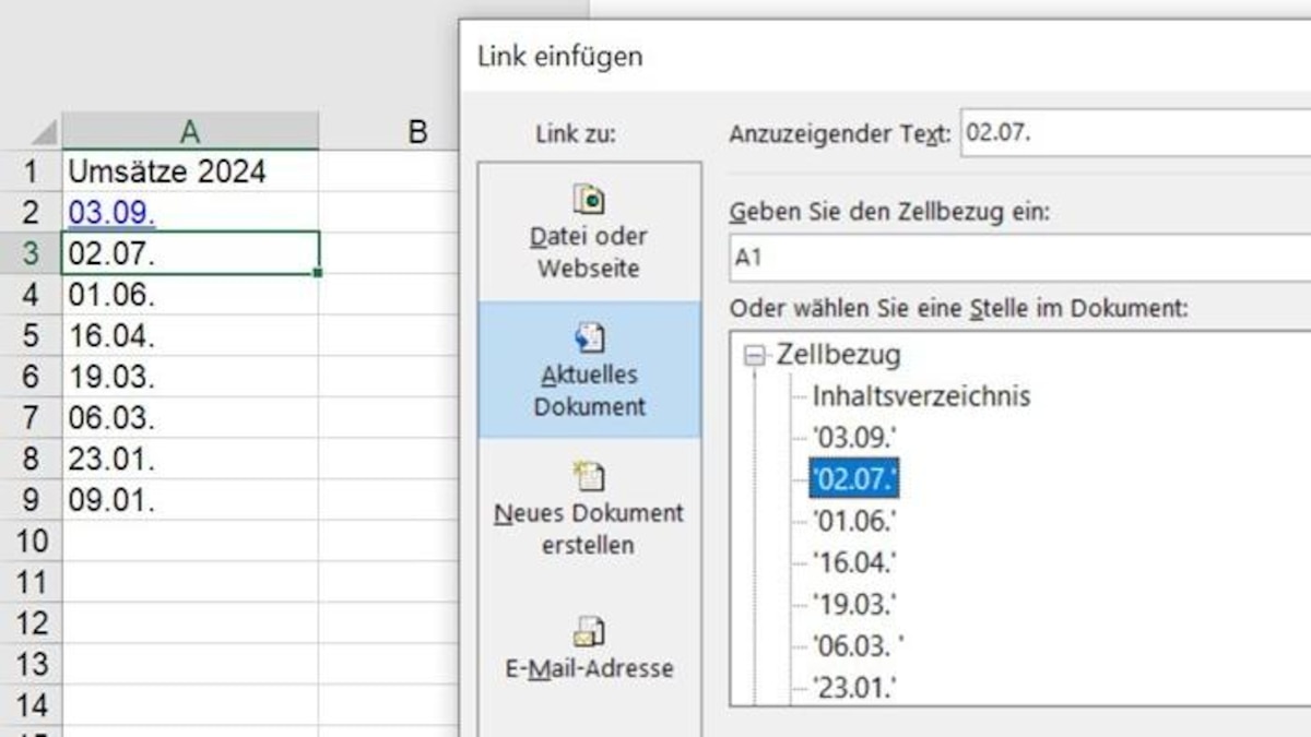
- In the dialog window on the left, select the source from which the link comes. In our example, this is “Current Document” (see Figure 2 below). Click the symbol once with the left mouse button.
- Under “Enter the cell reference:” you specify where the cursor should jump when you later open the worksheet via the link. By default, Excel always navigates to the first cell in the first column, i.e. A1.
- Now select the worksheet from the list that you want to switch to when you click later. In our example: “02.07”. Confirm your selection by clicking OK.
- Now click in cell A3 and repeat steps 6 – 9 for all worksheets in your Excel workbook. After you have inserted all the links, simply open the desired worksheet by clicking with the mouse.
Latest Videos
Create a table of contents for worksheets in an Excel workbook – Manual method (Image 1)
Create a table of contents for worksheets in an Excel workbook – Manual method (Image 1)
Create a table of contents for worksheets in an Excel workbook – link assignment is done via a dialog box (Figure 2)
Create a table of contents for worksheets in an Excel workbook – link assignment is done via a dialog box (Figure 2)
Create a table of contents using an Excel macro
If you find it too tedious to create the table of contents manually, you can also write a macro to do it. It will automatically create a list of all worksheets and insert hyperlinks to jump directly to the respective sheets. You can do this using the VBA developer tools.
- If the “Developer” tab is not displayed in your open workbook, activate it first. To do this, click on the “File” tab, select “More…” in the command column at the bottom left and then “Options”. Under “Customize the Ribbon”, check the box next to “Developer” and confirm with OK.
- Now you can access the Developer tab. Click on Visual Basic (first icon on the left). This will open the Visual Basic Editor.
- Paste the VBA code shown in the image below into the module. Then press Alt + Q to close VBA and return to Excel.
- The macro is called “CreateTableOfContents”. Call it by clicking the “Macros” icon from the “Developer Tools”. Highlight the macro name and click “Run”.
- Now call up any other worksheet you want by clicking on it from the new “Table of Contents” worksheet.